A new approach to modelling asset deterioration

Asset deterioration modelling is an important part of the toolkit for assessing asset health and improving asset performance. Currently used methods are based on quantifying asset health as a failure probability calculated from a failure distribution, for example Weibull, or as a measure of asset condition, for example wear of a critical component, and displayed in a P-F (potential failure – failure) curve.

This article describes how PAM Analytics uses survival analysis, a method commonly used in epidemiology, to develop descriptive asset deterioration curves and predictive asset deterioration models to gain insight and understanding into asset performance and so improve asset management. It is useful to note that survival analysis is used to analyse and model Covid infection and mortality data. The analogy between human condition (survival/death) and treatment, and asset condition (working/failure) and maintenance is clear.

Descriptive Asset Deterioration – Kaplan Meier Analysis

PAM Analytics uses Kaplan Meier (KM) analysis to produce descriptive asset deterioration curves. The output is the cumulative hazard and survival probability of each asset at time t. The cumulative hazard at time t is the cumulative risk of failure at time t and is related directly to survival probability (the probability of surviving to time t). Failure probability is given by 1-survival_probability.

KM analysis has two significant advantages over traditional failure distributions:

It is non-parametric, i.e. it does not make any assumptions about the data, for example that they follow a particular distribution.

It can quantify the effects of individual factors, for example asset specification and different types and levels of maintenance, on asset performance.

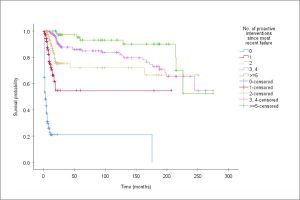
Figure 1 shows deterioration curves produced using KM analysis. The effects of different levels of proactive maintenance on asset survival probability are clear.

Hazard rate, also known as the conditional (instantaneous) failure rate function or hazard function, is another metric for assessing asset performance. It is the risk of failure at time t given that failure had not occurred by time t. Thus, the hazard rate at time t depends on the risk set at time t, i.e. the number of assets in use and therefore at risk of failure then.

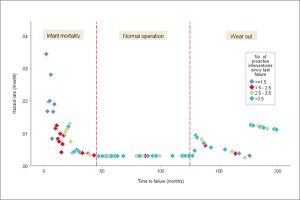
Hazard rate is arguably a better measure of reliability than failure probability because it considers the risk set at each time. As the number of failures decreases, the failure probability approaches the hazard rate. Figure 2 shows a hazard rate curve (the ‘bathtub’ curve) calculated from the cumulative hazard, and therefore as with the cumulative hazard no assumptions about the data were made.

To help understand hazard rate and cumulative hazard, Table 1 shows the analogy between hazard rate and cumulative hazard with speed and distance.

Table 1: Analogy of Hazard Rate and Cumulative Hazard with Speed and Distance

Predictive Asset Deterioration – Cox Regression

KM analysis can be viewed as the exploratory data analysis stage of developing predictive Cox regression models. The models are at individual asset level and have a dynamic component and a static component. The dynamic component shows how the risk of failure increases as assets are used. The static component contains the predictors. Table 2 shows the predictors and coefficients of a Cox regression deterioration model for wet well submersible pumps.

Table 2: Example Cox Regression Predictive Asset Deterioration Model (static component)

The main conclusions from Table 2 are that proactive maintenance has the greatest effect on reducing the risk of asset failure (Figure 1 has a similar conclusion about the extent of proactive maintenance) and that a history of repeated asset failure increases the risk of future failure. They confirm accepted practice but the model goes further by calculating the risk of failure of each asset as it is used, maintained, fails and then reinstated.

Dr Atai Winkler, PAM Analytics

atai.winkler@pamanalytics.com